Day 8
Today
- Dictionaries and Tuples
- Memoization
- More Recursion Practice
- Studio time
For next time
- This week’s reading is longer than usual as we dive into Classes. Be sure to budget time for active reading and use NINJA hours throughout the week.
Survey Takeaways
-
Your honest answers help us keep your workload in the sweetspot, where we are not burying you or boring you. On average, MP1 seems to be on the higher end of challenging but close to the middle for hours spent.
-
We collect information about the structure of the MP and RJs - and consider them for how we scaffold future versions of the same assignment next semester (and when appropriate we use our learnings as we release subsequent RJs and MPs).
-
We learn how people are utilizing the help structures, such as NINJAs.
-
This is a class where students can drive at their own desired speed, we see people who had familiarity with the programming concepts in MP1 challenging themselves.
-
The amount of Python scaffolding for MP1 seems appropriate, but we could use some more time spent on the biological concepts studied.
Reading Journal Debrief
Now that we’ve read about Dictionaries and Tuples, we’ve seen almost all built-in Python types. As an activity, let’s compare and contrast the types and their uses.
With the person sitting next to you, review your solutions to the most_frequent exercise. Pay particular attention to your strategies for iteration and sorting.
“Recursive” problem analysis from 5 Whys, introduction and Examples and An Introduction to 5-why: What is the value in continuing to ask “why”? How do you know when you’ve reached a root cause?
Recursion Practice
Levenshtein Distance
Let’s circle back on some of the recursion practice problems from last time. We’ll start by implementing Levenshtein distance together as a class. Here is the description of the problem from last time.
Write a function called levenshtein_distance that takes as input two strings
and returns the Levenshtein
distance between the two
strings. Intuitively, the Levenshtein distance is the minimum number of edit
operations to transform one string into the other (for this reason Levenshtein
distance is sometimes called “edit distance”). These edits can either be
insertions, deletions, or substitutions. Note that Levenshtein distance is
similar to Hamming distance,
but works for strings of differing lengths
Here are some examples of these operations:
- kitten → sitten (substitution of
sfork) - sitten → sittin (substitution of
ifore) - sittin → sitting (insertion of
gat the end).
While this function seems initially daunting, it admits a very compact recursive solution. You can either work on your own to see the recursive solution, or use the recursive solution given in the Wikipedia article.
To get a better handle on this, let’s consider some more examples.
levenshtein_distance('kitten', 'smitten') -> 2 (see below for steps)
- kitten → sitten (k gets replaced by s)
- sitten → smitten (insert between s and i)
levenshtein_distance('beta', 'pedal') -> 3 (see below for steps)
- beta → peta (b gets replaced by p)
- peta → petal (l gets inserted at the end)
- petal → pedal (t gets replaced by d)
levenshtein_distance('battle', 'bet') -> 4 (see below for steps)
- battle → bettle (a gets replaced by e)
- bettle → bettl (the last e gets deleted)
- bettl → bett (delete l)
- bett → bet (delete t)
Base Cases
Let’s consider the base cases when one of the two strings is empty. What should the Levenshtein distance be in this case?
Recursive Step
Let’s consider the different ways in which we can make the first character of string a equal to the first character of string b. Here are the possible cases.
- The first two characters are already equal
- Replace the first character of string a with the first character of string b
- Insert the first character of string b before the characters of string a
- Delete the first character of string a
For each of these steps we have to consider two things:
- How much does this first step cost?
- How much does it cost to make the rest of the two strings equal to each other
Let’s write a recursive implementation of this function.
Memoization
Last class, a lot of you had the chance to do this exercise:
Write a function called choose that takes two integer, n and k, and returns
the number of ways to choose k items from a set of n (this is also known as
the number of combinations of k
items from a pool of n). Your solution should be implemented recursively using
Pascal’s rule.
Here is a sample solution:
def nchoosek(n, k):
    """ returns the number of combinations of size k
        that can be made from n items.

        >>> nchoosek(5,3)
        10
        >>> nchoosek(1,1)
        1
        >>> nchoosek(4,2)
        6
    """
    if k == 0:
        return 1
    if n == k:
        return 1
    return nchoosek(n - 1, k - 1) + nchoosek(n - 1, k)

if __name__ == '__main__':
    import doctest
    doctest.testmod(verbose=True)
It passes all the unit tests!!! Hooray!
Unfortunately, this code is going to be quite slow. To get a sense of it, let’s draw a tree that shows the recursive pattern of the function.
You can even visualize the call graph within Jupyter notebook using an extension. In Linux:
$ sudo apt-get install graphviz
$ pip install callgraph
Then within your notebook, you can draw a call graph as a function is called:
%load_ext callgraph
%callgraph nchoosek(4, 2)
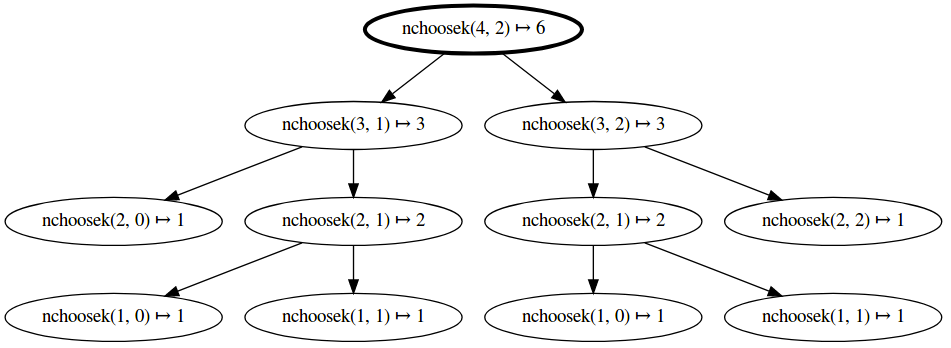
As you can see, the function is recursively called multiple times with the same arguments.
In order to improve the speed of this code, we can make use of a pattern called memoization. The basic idea is to transform a recursive implementation of a function to make use of a cache (in this case a Python dictionary) that remembers all previously computed values for the function. Here’s is a skeleton of a memoized recursive function (we are being a little fast and loose with the mixing pseudo code and Python, but this should become clearer as you do a concrete example.
def recursive_function(input1, input2):
    if input1, input2 is a base case:
        return base case result
    if input1, input2 is in the list of already computed answers
       return precomputed answer
    return recursive step on a smaller version of input1, input2
Add memoization to your implementation of nchoosek (and/or levenshtein_distance) and study its impact on performance.
Think Python Chapter 11.6 will also be helpful.
Turtle World
We’re devoting a bit more time to Turtle World today - with the remainder of the time, choose at least one of the fractal drawings below to pursue.
One additional bit of fun: now that we know about tuples, we’re not limited to a tiny color palette. Colors in computer graphics are typically expressed as a (red, green, blue) tuple, which you can pass to turtle.color to paint the entire rainbow!
Teleportation, Cloning, and Other Unethical Experiments on Turtles
In addition to the what you did on your day 5 reading journal and in the day 6 class activity, a few other Turtle Tricks that may prove useful.
A Turtle is a Python object, which we will learn more about next week. Turtles
have methods, which we can call to inspect change their behavior. One trick that will be useful here, which you saw in shapes.py but may not have thought about much, is the speed() function. The speed() function can be used to speed up slowpoke Turtles. While it seems weird that a speedy turtle would have a speed of 0, in this case the input 0 is reserved for having the turtle go as fast as possible (remember, when in doubt, check the documentation).
import turtle
speedy = turtle.Turtle()
speedy.speed(0)
Other important Turtle methods include xcor() and ycor() position, and
heading().
Read more about turtles here.
Since Turtles are simple creatures, mainly defined by their current position and heading, we can “clone” them by reading these values and using them to direct a new Turtle.
leo = turtle.Turtle()
# leo does some arbitrary drawing (e.g., makes a 45 degree angle)
leo.fd(100)
leo.lt(45)
leo.fd(100)

# Create a new Turtle with the same attributes as the first
don = turtle.Turtle()
don.penup()
don.setx(leo.xcor())
don.sety(leo.ycor())
don.setheading(leo.heading())
if leo.isdown():
    don.pendown()
# don.bandana_color = "purple" # TODO: Ninja functionality not yet implemented
As an exercise, encapsulate this functionality in a clone function that
takes a Turtle argument and returns a new Turtle with the same position
and heading, leaving the original Turtle untouched.
Fractals
Fractals are geometrical constructions that display self-similar repeated patterns at every scale as you zoom in. They are often extremely beautiful, and are found throughout nature. Fractals are also useful across many fields, from antenna engineering to poetry to finance. Check out Yale’s Panorama of Fractals and their Uses for more examples.
Today, we will teach our turtles to draw fractal shapes using recursion. A
very cool recursive drawing we can create is called the snowflake curve (or
Koch snowflake). To get
started, let’s write a function called snow_flake_side with the following
signature:
def snow_flake_side(turtle, length, level):
    """Draw a side of the snowflake curve with side length length and recursion
    depth of level"""
The snow_flake_side function should have a base case that draws the following image:
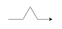
The recursive step should replace each of the line segments above with a
snow_flake_side with size length / 3.0 and recursion depth level - 1. Take
some time to work on this and then we’ll discuss as a group.
Once you have completed your snow_flake_side function, create a function
called snow_flake that draws the whole snowflake.
Recursive Trees
Next, we will draw a tree using recursion. Define a function called
recursive_tree that takes as input a turtle, a branch length, and a
recursion depth and draws the recursive tree to the canvas.
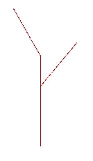
def recursive_tree(turtle, branch_length, level):
    """Draw a tree with branch length branch_length and recursion depth of level
    """
The base case is:

This structure is given by moving forward branch_length steps (assuming the
turtle has the correct orientation).
For the recursive step, you should:
- Draw the line as above
- Clone your turtle
- Turn the new turtle left 30 degrees
- Recurse using the cloned turtle to draw a tree with branch length
branch_length * 0.6and depth `level - 1 - Hide the cloned turtle using the
hideturtlemethod - Back the original turtle up
branch_length / 3.0 - Clone your turtle
- Turn the new turtle right 40 degrees
- Recurse using the cloned turtle to draw a tree with branch length
branch_length * 0.64and depthlevel - 1 - Hide the cloned turtle using the
hideturtlemethod
After implementing the recursive step, if you set level to 1 more than the
base case (which will either be 1 or 2 depending on what level you consider
the base case), you will get the following picture:
Once you’ve built your recursive_tree function, try making a few
enhancements:
- Make the base case change the pen color for the turtle to green (this will simulate the appearance of leaves if you do a high enough depth)
- Add some randomness to the degree of left turn, right turn, and scaling so that you get more naturalistic looking trees
- Add more than two branches
More Recursion
The Koch snowflake and our recursive tree are both part of a more general class of curves called L-systems (Lindenmayer Systems). Next, read the linked Wikipedia article on L-systems and try to implement Sierpinski’s triangle and fractal plant.
Hint 1: For Sierpinski’s triangle you will want to create a function to generate both symbols A and B and have them call each other.
Hint 2: For the fractal plant you should create the following functions to
save and then restore then Turtle’s state (symbols [ and ] respectively):
def save_turtle_state(turtle_states, t):
    turtle_states.append((t.xcor(), t.ycor(), t.heading()))

def restore_turtle_state(turtle_states, t):
    s = turtle_states.pop()
    t.penup()
    t.setx(s[0])
    t.sety(s[1])
    t.setheading(s[2])
    t.pendown()